Fast Inverse Square Root Algorithm Explained

Why we need a fast inverse square root algorithm
The inverse square root means
In the field of Computer Graphics, the inverse square root of a number is usually used for normalizing vectors. As this operator is used a lot, deriving a fast algorithm for it becomes very important.
Algorithm itself
float Q_rsqrt(float number) {
    long i;
    float x2, y;
    const float threehalfs = 1.5F;

    x2 = number * 0.5F;
    y = number;
    i = *( long * ) &y;                      // evil floating point bit hack
    i = 0x5f3759df - (i >> 1);               // what the fuck?
    y = * (float * ) &i;
    y = y * ( threehalfs - (x2 * y * y) );   // 1st iteration
//  y = y * ( threehalfs - (x2 * y * y) );   // 2nd iteration, can be removed
    return y;
}
Intuitions behind this algorithm
Use multiply instead of division in code
In general, computing the division between two numbers are much more costly than multiplying two numbers together in computer. This can be easily verified by running the following C program.
#include <stdio.h>
#include <time.h>
#include <stdlib.h>


const int sz = 1 << 20;
const int trail = 100;

int main() {
    clock_t start, end;
    float * arr1 = (float*)malloc(sizeof(float) * sz);
    float * arr2 = (float*)malloc(sizeof(float) * sz);
    float * arr3 = (float*)malloc(sizeof(float) * sz);

    /*
    In order to avoid the timing inconsistency caused by 'cold cache', we need to access every
    single elements inside the arrays we use for performance profiling.
    */
    for (int i = 0; i < sz; ++i) {
        arr1[i] = (float)rand() / (float)RAND_MAX;
        arr2[i] = (float)rand() / (float)RAND_MAX;
        arr3[i] = 0;
    }

    double time_used_multiply = 0;
    double time_used_division = 0;

    /*
    To avoid our code any unnecessary optimization provided by compiler, we do multiplication job
    and division job alternativly in each profiling loop.
    */

    for (int t = 0; t < trail; ++t) {
        start = clock();
        for (int i = 0; i < sz; ++i) {
            arr3[i] = arr1[i] * arr2[i];
        }
        end = clock();
        time_used_multiply += ((double) (end - start)) / CLOCKS_PER_SEC;

        start = clock();
        for (int i = 0; i < sz; ++i) {
            arr1[i] = arr3[i] / arr2[i];
        }
        end = clock();
        time_used_division += ((double) (end - start)) / CLOCKS_PER_SEC;
    }
    time_used_multiply /= trail;
    printf("Average time used for multiplication job: %f\n", time_used_multiply);
    time_used_division /= trail;
    printf("Average time used for division job: %f\n", time_used_division);
}
Average time used for multiplication job: 0.001960
Average time used for division job: 0.005490
As division is much more costly than computing multiplication, we want to minimize the number of occurance of division operators.
Try not to use the sqrt() function
The cost of sqrt() can be estimated using the following C program.
#include <stdio.h>
#include <time.h>
#include <stdlib.h>
#include <math.h>


const int sz = 1 << 20;
const int trail = 100;

int main() {
    clock_t start, end;
    float * arr1 = (float*)malloc(sizeof(float) * sz);
    float * arr2 = (float*)malloc(sizeof(float) * sz);

    for (int i = 0; i < sz; ++i) {
        arr1[i] = (float)rand() / (float)RAND_MAX * 1024;
        arr2[i] = 0;
    }

    double time_used = 0;

    for (int t = 0; t < trail; ++t) {
        start = clock();
        for (int i = 0; i < sz; ++i) {
            arr2[i] = sqrt(arr1[i]);
        }
        end = clock();
        time_used += ((double) (end - start)) / CLOCKS_PER_SEC;
    }
    time_used /= trail;
    printf("Average time used for sqrt job: %f\n", time_used);
}
Average time used for sqrt job: 0.004730
Algorithm explained
Newton’s Method
Newton’s method can be used to find a root of a function in an iterative manner. Therefore, we can convert the problem of computing
We want to find a
Using Newton’s method to derive the iterative routine for the problem:
In order to achieve desired accuracy with minimum number of iterations needed, we want our initial guess of
Floating point number
According to IEEE 754, floating point number is represented by 32 bits in the following manner.

For detailed description about this representation, can take a look at this.
In general, the first bit represent the sign of the number, 0 for positive while 1 for negative.
The unsigned number
The remaining 23 bits are used to represent the mantissa of the floating point number, as scientific representation requires the first digit of the number to be non-zero, the value for the first digit of mantissa in the binary representation can only be 1. Therefore, we can save this digit for higher accuracy representation.
In the end, the value of the number behind the scene is:
Dark Magic
Take the logarithm of the number, we will get:
As
A good approximation for the function would be the following function:
Apply the approximation to the formula above:
Notice here, we have
We also have the following relationship:
Therefore, the WTF line in the code seems to be clear at this stage. The -(i>>1) term is calculating 0x5f3759df in front of this term should be the value of
#include <stdio.h>

int main() {
    long target = 0x5f3759df;
    long a = 3 * (1 << 22) * 127;
    long b = 3 * (1 << 22) * 0.0430;
    double mu = (double)(a - target) / (3 * (1 << 22));
    printf("%e\n", mu);
    printf("%08lx\n", a - b);
    printf("%08lx\n", target);
}
4.504657e-002
5f37be77
5f3759df
We can see that the value of
Assemble everything together
After all these efforts, we finally get the binary representation of the number approximate value of
Error Estimation and Performance Profiling
The error of the algorithm is estimated over the entire domain of float using log-space grid. Here is the code and output of this profiling process.
#include <stdio.h>
#include <math.h>
#include <float.h>
#include <time.h>
#include <stdlib.h>

void logspace(float start, float end, int n, float* u) {
    float pow_start = log2f(start);
    float pow_end = log2f(end);
    float step = (pow_end - pow_start) / (n - 1);
    for (int i = 0; i < n; ++i) {
        u[i] = powf(2, pow_start + i * step);
    }
}

static inline float Q_rsqrt(float y) {
    long i;
    float x2;

    x2 = y * 0.5F;
    i = 0x5f3759df - ((*( long * ) &y) >> 1);               // what the fuck?
    y = * (float * ) &i;
    y *= ( 1.5F - (x2 * y * y) );   // 1st iteration
//  y *= ( 1.5F - (x2 * y * y) );   // 2nd iteration, can be removed
    return y;
}

int main() {
    int profiling = 1;
    int trail = 100;
    int sz = 1 << 20;
    float * xs = (float*)malloc(sizeof(float) * sz);
    logspace(FLT_MIN, FLT_MAX, sz, xs);
    float * result = (float*)malloc(sizeof(float) * sz);
    float * ground = (float*)malloc(sizeof(float) * sz);
    for (int i = 0; i < sz; ++i) {
        result[i] = Q_rsqrt(xs[i]);
    }

    for (int i = 0; i < sz; ++i) {
        ground[i] = 1 / sqrt(xs[i]);
    }

    if (profiling) {
        double quick_alg_time = 0;
        double orig_alg_time = 0;
        clock_t start, end;
        for (int t = 0; t < trail; ++t) {

            for (int i = 0; i < sz; ++i) {
                result[i] = 0;
            }

            for (int i = 0; i < sz; ++i) {
                ground[i] = 0;
            }

            start = clock();
            for (int i = 0; i < sz; ++i) {
                result[i] = Q_rsqrt(xs[i]);
            }
            end = clock();
            quick_alg_time += ((double) (end - start)) / CLOCKS_PER_SEC;

            start = clock();
            for (int i = 0; i < sz; ++i) {
                ground[i] = 1 / sqrt(xs[i]);
            }
            end = clock();
            orig_alg_time += ((double) (end - start)) / CLOCKS_PER_SEC;
        }
        quick_alg_time /= trail;
        printf("Average time used for quick algorithm: %f\n", quick_alg_time);
        orig_alg_time /= trail;
        printf("Average time used for naive approach: %f\n", orig_alg_time);
    }

    FILE* output_f = fopen("output.bin", "wb");
    if (fwrite(xs, sizeof(float), sz, output_f) != sz) {
        perror("Cannot write to file!");
        return 1;
    }
    if (fwrite(result, sizeof(float), sz, output_f) != sz) {
        perror("Cannot write to file!");
        return 1;
    }
    if (fwrite(ground, sizeof(float), sz, output_f) != sz) {
        perror("Cannot write to file!");
        return 1;
    }
}
Average time used for quick algorithm: 0.004890
Average time used for naive approach: 0.005990
import struct
import numpy as np
import matplotlib.pyplot as plt

sz = 1 << 20

with open("./output.bin", "rb") as f:
    form = "f" * sz
    xs = np.array(struct.unpack(form, f.read(struct.calcsize(form))))
    results = np.array(struct.unpack(form, f.read(struct.calcsize(form))))
    grounds = np.array(struct.unpack(form, f.read(struct.calcsize(form))))

plt.loglog(xs, np.abs(grounds - results), base=2)
plt.show()
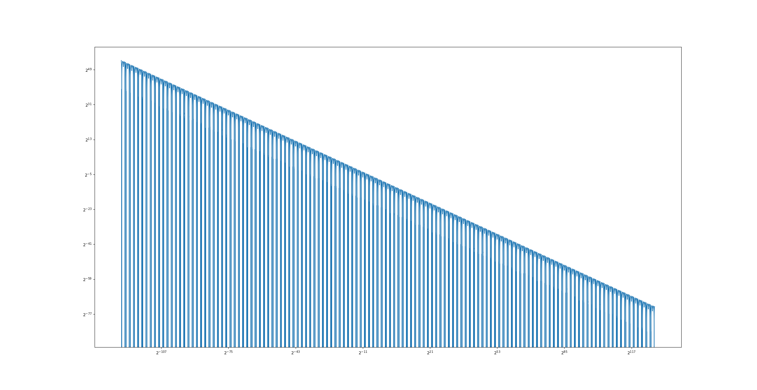
From the output we can see that even with my naive implementation of the quick inverse square root algorithm, the algorithm still out performs the naive approach.
The error of the algorithm is acceptable for
Reference
- Youtube Video “Fast Inverse Square Root — A Quake III Algorithm”
https://www.youtube.com/watch?v=p8u_k2LIZyo
Study Notes For Fractional Calculus I
Fractional derivative for polynomialIn most cases, when we are calculating different orders of de...
A Short Proof Showing Why (1-x)(1+x) Is Different From (1-x^2) During Computation
When computing , we know that catastrophic cancellation may happen when we are computing the minu...